I wanted to outfit my Raspberry Pi (which will be used for a UAV flight controller and data recorder) with the new 64-bit operating system and the PREEMPT_RT kernel patch.
Basically, PREEMPT_RT allows user-space code to preempt operating system tasks. The “real time” designation doesn’t necessarily guarantee faster operation, but it does guarantee the predictable and timely execution of user tasks, as they cannot be deferred by the OS. In general, the OS does a good enough job of scheduling tasks for a smooth user experience, but in the case of robotics or instances where precise timing or the immediate handling of interrupts is required, a more rigid scheduling regime is necessary. The PREEMPT_RT patch modifies the Linux kernel to enable this.
So, here’s realtime, 64-bit Linux on RPi 4, the easy way (cross-compiling on Linux):
- Download the 64-bit Raspbery Pi OS image. (It’s under development as of this date, so this link will become obsolete soon.)
- Install the image onto a microSD card using the Raspberry Pi Imager. (Available through apt as rpi-imager on systems that use it.)
- Follow the kernel-building instructions given by the Raspberry Pi Foundation for the 64-bit operating system (kernel8). However:
- After cloning the kernel repository, CD into the repo and download the correct version of the PREEMPT_RT patch into it. Note that the patch version must match the kernel version. In my case the kernel was at 5.4.70 and the patch was at 5.4.69. It worked, but this is never guaranteed. If the patch isn’t up to date with the kernel, check out an older kernel.
- Apply the patch using the command:
zcat patch-5.4.69-rt39.patch.gz | patch -p1 - Execute
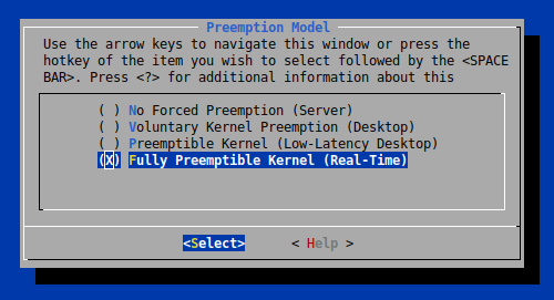
make menuconfig. When the menu opens, navigate toGeneral setup ---> Preemption Modeland selectFully Preemptible Kernel (Real-Time)(see screenshot below). High-precision timers are also required, but are already selected. Remember to save the configuration and exit out of the menu. - Continue with the kernel-building instructions where you left off at #4.
To make life easier, enable ssh on the Pi by executing touch /path/to/boot/ssh. This places an empty file called ssh in the boot partition which enables ssh so you can hook the Pi up to your network and log in without attaching a keyboard and monitor. From there, complete the configuration using raspi-config.
When you boot into your system, check that the patched kernel has been loaded by executing the command, uname -a. You should see something like the following:

The “PREEMT” string tells you the correct kernel has been loaded.
Here’s a script I use to build and install the kernel and patch. It will ask for the boot (Fat32) and rootfs (Ext4) device partitions, which will be something like /dev/sdf1 and /dev/sdf2. You can find these using lsblk.
As always, no warranty is expressed or implied. Be very careful when selecting the devices to write to and back up your data first!
![\[S(x) = p \sum_{i=1}^{n} \left( \frac{(Y_i - \hat{f}(x_i))^2}{\sigma_i^2} \right) + (1 - p) \int{ \left( \hat{f}^{(m)}(x) \right)^2 } dx,\]](https://robskelly.com/wp-content/ql-cache/quicklatex.com-58d58ad969d57dd3193e187e43cc9033_l3.png "Rendered by QuickLaTeX.com")
 , the weight, from
 ![[0,1]](https://robskelly.com/wp-content/ql-cache/quicklatex.com-25b6d943ab489c05a3dbd5ea29087a48_l3.png "Rendered by QuickLaTeX.com") , is applied to the first term (the least squares part), and its negation is applied to the second term (the integral part). The denominator of the least squares term is a weight for which the FITPACK documentation suggests the reciprocal of the standard deviation. In that case, the smoothing factor is recommended to be in the vicinity of
, is applied to the first term (the least squares part), and its negation is applied to the second term (the integral part). The denominator of the least squares term is a weight for which the FITPACK documentation suggests the reciprocal of the standard deviation. In that case, the smoothing factor is recommended to be in the vicinity of  . One may also choose a variable weight.