The Power Function
It’s time to get to the heart of this application.
Martin, Milliken and Cobb (1998) documented an amazingly comprehensive cycling power model using a wind tunnel and SRM power meter for validation. Their model considers tangent winds, wheel bearing and wind drag, power loss through changes in kinetic energy, gradient, etc. The model makes some assumptions that may not be realistic for a general audience. For example, all of the subjects were young men, experienced cyclists, riding racing bikes. The functions derived for estimating the riders’ frontal area are derived from a relatively small, uniform sample of the cycling population, the wheel bearing drag is derived from very high-quality equipment in good trim, and the spoke drag is estimated from time trial wheels, which are much more slippery than standard road wheels.
However, the model is a great starting point, and matches the power readings of the SRM convincingly. If functions or constants for some of these coefficients are available, I can add those refinements later. For example, it would be nice to have a frontal-area model that considers gender, and is not based only on whippet-thin young men.
The power function follows:
![P_{tot} = [V_{a}^2 V_{g} 1/2 \rho (C_{d} A + F_{w}) + V_{g} C_{rr} m g \cos(\arctan(G_{r})) + V_{g} (91 + 8.7 V_{g}) 10^-3 + V_{g} m g \sin(\arctan(G_{r})) + 1/2 (m + I/r^2) (v_{f}^2 - v_{i}^2) / (t_{f} - t_{i})] / E_{c}](https://s0.wp.com/latex.php?latex=P_%7Btot%7D+%3D+%5BV_%7Ba%7D%5E2+V_%7Bg%7D+1%2F2+%5Crho+%28C_%7Bd%7D+A+%2B+F_%7Bw%7D%29+%2B+V_%7Bg%7D+C_%7Brr%7D+m+g+%5Ccos%28%5Carctan%28G_%7Br%7D%29%29+%2B+V_%7Bg%7D+%2891+%2B+8.7+V_%7Bg%7D%29+10%5E-3+%2B+V_%7Bg%7D+m+g+%5Csin%28%5Carctan%28G_%7Br%7D%29%29+%2B+1%2F2+%28m+%2B+I%2Fr%5E2%29+%28v_%7Bf%7D%5E2+-+v_%7Bi%7D%5E2%29+%2F+%28t_%7Bf%7D+-+t_%7Bi%7D%29%5D+%2F+E_%7Bc%7D+&bg=ffffff&fg=000000&s=0 "P_{tot} = [V_{a}^2 V_{g} 1/2 \rho (C_{d} A + F_{w}) + V_{g} C_{rr} m g \cos(\arctan(G_{r})) + V_{g} (91 + 8.7 V_{g}) 10^-3 + V_{g} m g \sin(\arctan(G_{r})) + 1/2 (m + I/r^2) (v_{f}^2 - v_{i}^2) / (t_{f} - t_{i})] / E_{c}")
Breaking it down a bit:
 is the ground velocity, what one would measure with a mechanical speedometer.
 is the air velocity of the bicycle in motion, found by adding the raw ground velocity to the tangential air velocity,
  which itself is found by
 ![V_{w} [\cos(D_{w} - D_{b})]](https://s0.wp.com/latex.php?latex=V_%7Bw%7D+%5B%5Ccos%28D_%7Bw%7D+-+D_%7Bb%7D%29%5D&bg=ffffff&fg=000000&s=0 "V_{w} [\cos(D_{w} - D_{b})]") , where
, where  is the wind velocity,
  is the wind direction, and
  is the bicycle’s direction of travel.
 is the air density, found by computing,
  , where
  is the partial pressure of dry air,
  is the pressure of water vapour,
  is the temperature (K),
  is the specific gas constant for dry air (287.058 J/(kg·K)) and
  is the specific gas constant for water vapor, (461.495 J/(kg·K)).
 is the coefficient of drag for a cyclist.
 is the projected frontal area of the cyclist.
 is the incremental area of the spokes of the wheel.
 is the coefficient of rolling resistance.
 is the mass of the rider and bike together.
 is the acceleration of gravity (approximately
  ).
). is the road gradient expressed as a fraction (rise/run).
 is the moment of inertia of the wheels (
 , used in this study).
 and
and  are the final and initial velocities of the segment being computed (m/s).
 and
and  are the final and initial times of the segment being computed (s).
 is the chain efficiency factor, which accounts for mechanical friction in the drive train of the bicycle.
The beautiful thing about this function, other than its accuracy — at least under the conditions of Martin, et al. — is that it can be built up incrementally using the data collected by the application, known constants, and a few estimates and functions found by the authors.
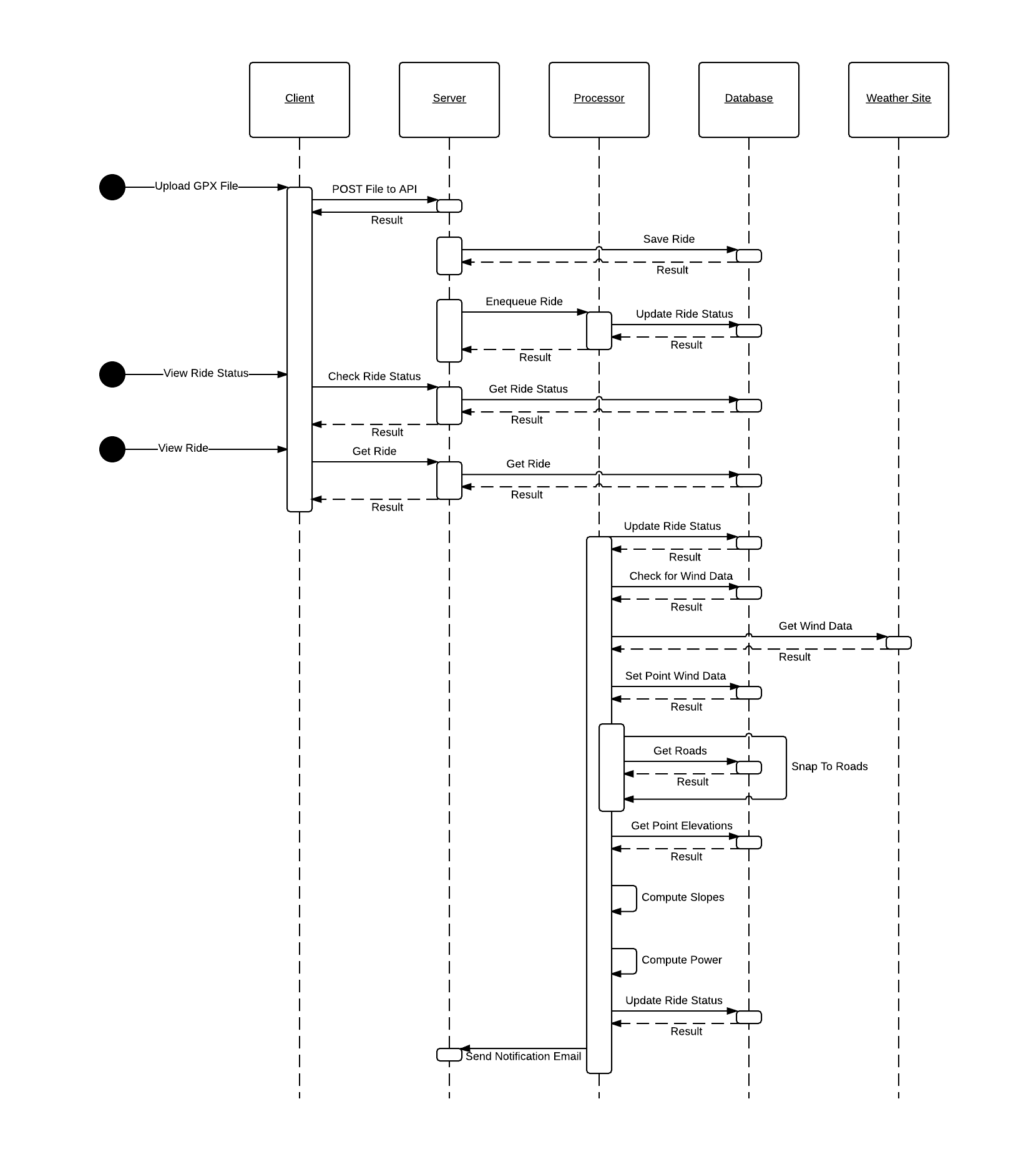
The Algorithm
The current high-level algorithm (provisional, until it reaches production!) is as follows:
- Begin by loading the required data.
- Load the rider’s characteristics.
- Load the bike’s characteristics.
- Load the ride’s characteristics.
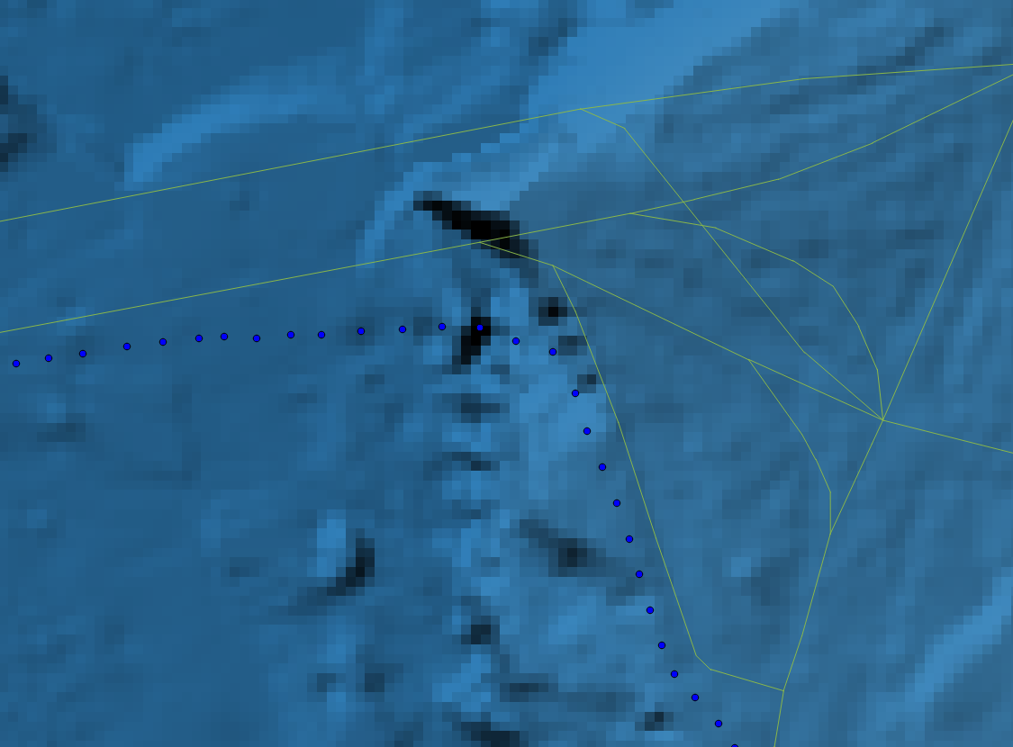
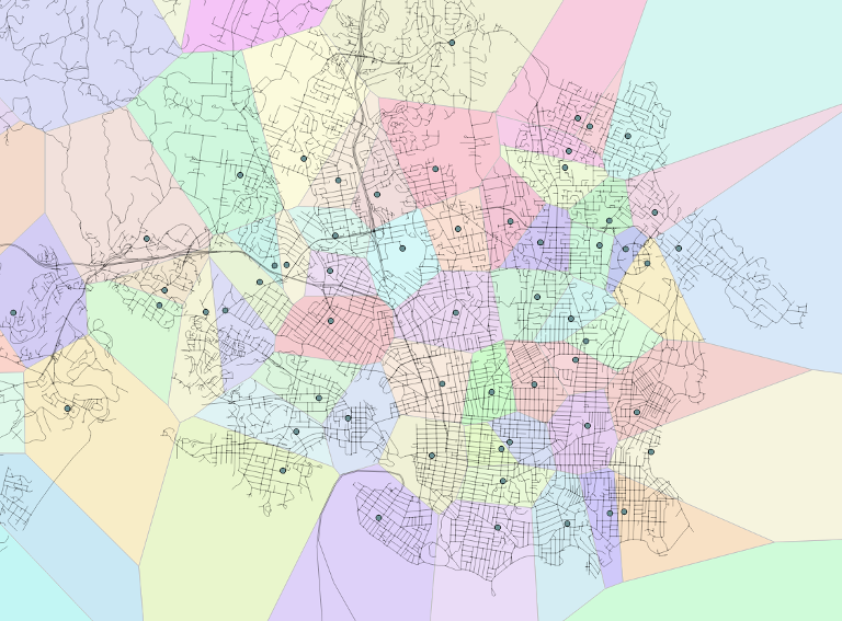
- Load the set of schools whose Voronoi cells intersect with the ride.
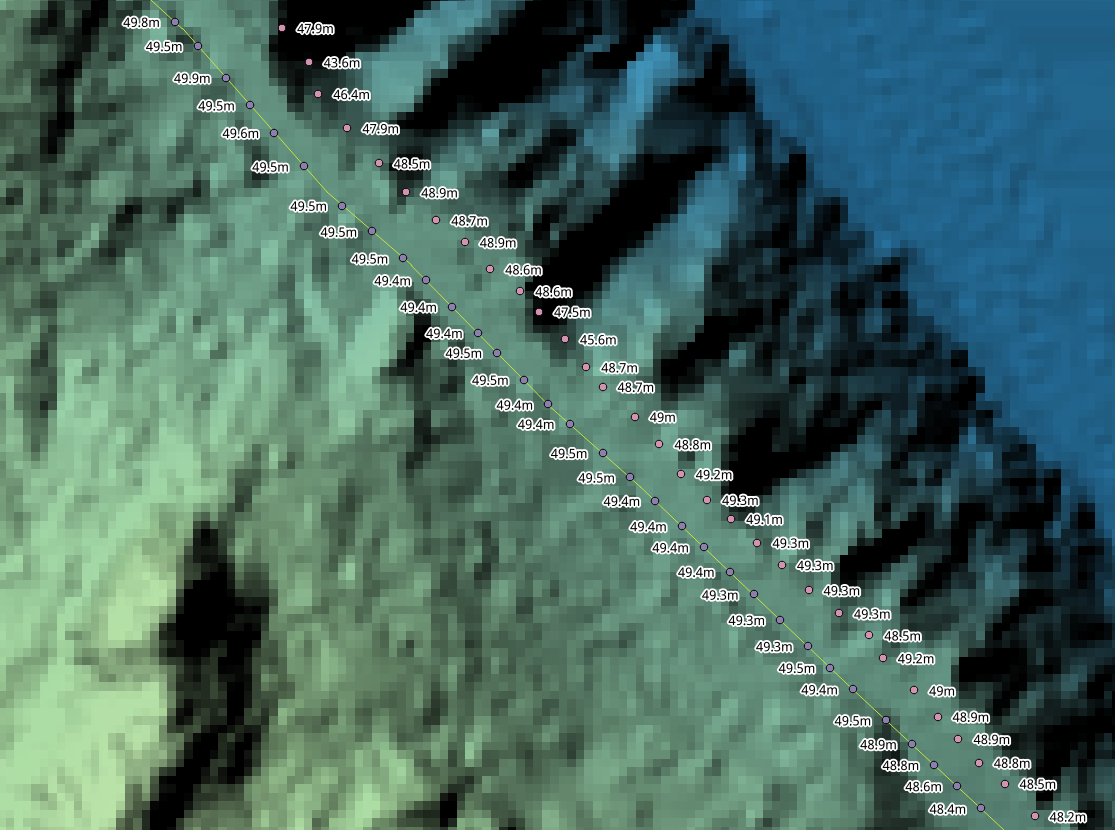
- Load the ride points, using a series of joins on the school, weather and DEM tables to retrieve the point’s time and location, along with the weather conditions for the point, the elevation and the slope.
- Iterate over the points, applying the power function to each one.
The Parameters
The Rider
The rider’s characteristics are entered when the user registers. The most important is the rider’s mass, but if there’s a way to include age and gender, those would be loaded too.
The Bike
The bike characteristics are mass and type, though the model as documented only supports road bikes.
The Ride
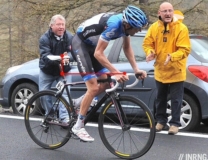
Hesjedal in the Drops
The model uses parameters that are deduced from the rider’s position — on the “tops,” on the “hoods” or in the “drops” — which has a large effect on their frontal area. The photo at right shows Victoria professional cyclist Ryder Hesjedal climbing in the hoods position. The photo illustrates a curious problem with modelling the air drag of riders. He is very tall for a professional cyclist (6’2″, like me, but about 15kg lighter!), but rides a tiny frame with a very large drop between the saddle and handle bars. A typical rider is much more upright in this position.
A rider never maintains one position over an entire ride, but it would be onerous to manually tell the application what position was being used at each segment (as if anyone could remember that anyway). Should the rider enter the position they use most (usually on the hoods), or should they attempt to estimate what percentage of the ride they spend in each position? Should the rider even be given the option to choose? Once I decide this, this information will be stored as an attribute of the ride. A the most likely default is the hoods position.
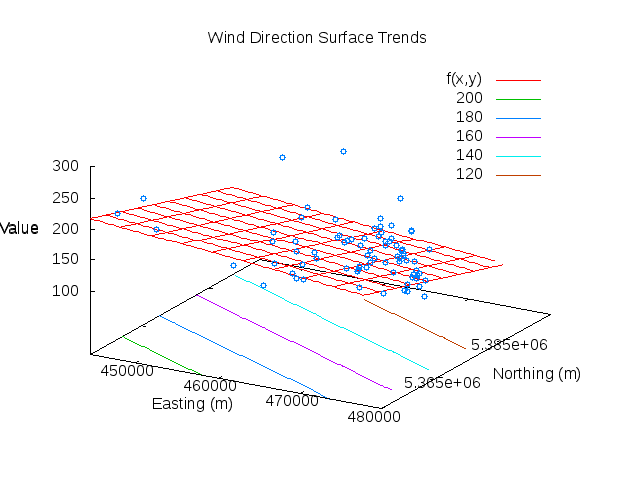
The School and Weather
The power function depends on wind speed and direction, but it also depends on the air density, which requires the air pressure, temperature and humidity. Counter-intuitively, perhaps, humid air is less dense than dry air, because the molar mass of a water molecule is lower than those of Oxygen and Nitrogen (Water is a single Oxygen with two Hydrogens; The Hydrogens are much lighter than the extra Oxygen on a molecule of Oxygen).
To accurately calculate the air temperature and pressure at the elevation of a ride point, the elevation of the school must be used to adjust its weather metrics to sea level, and then to the elevation of the cyclist.
The Points
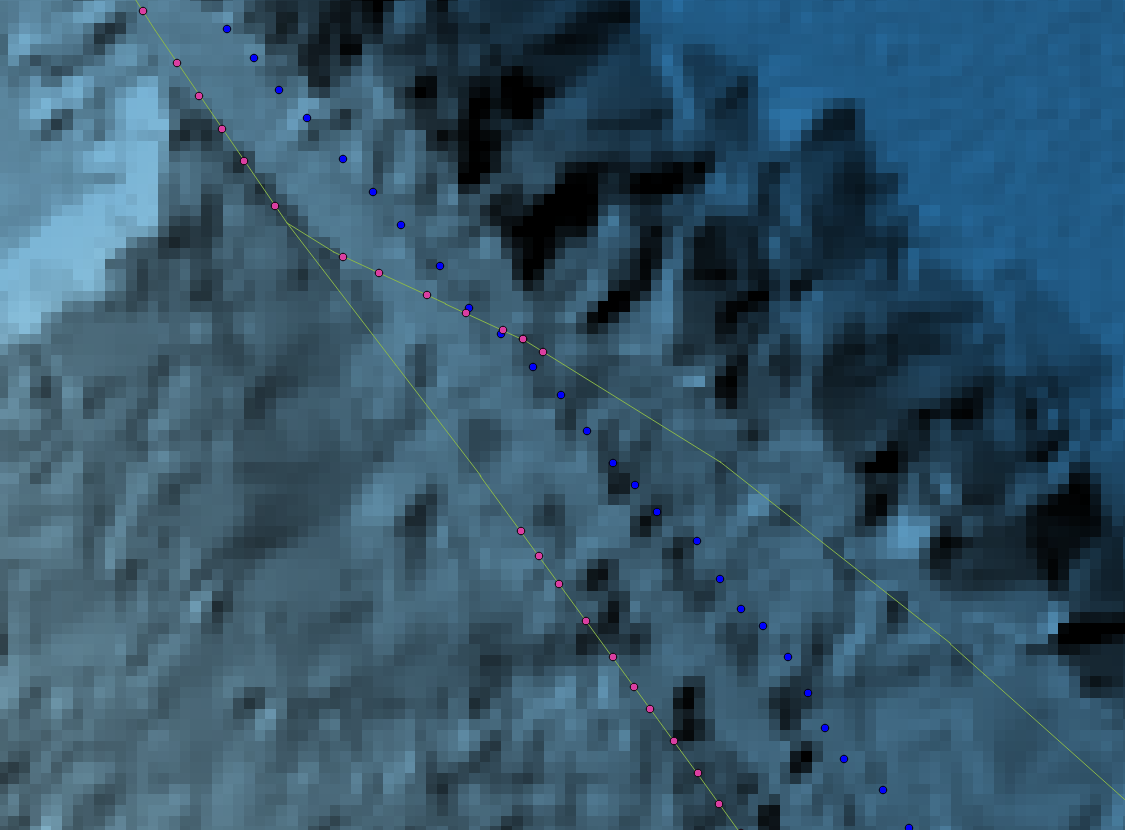
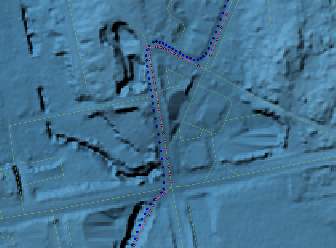
To parameterize the function the ride points must be traversed in chains of 3. This is because the time and velocity must be known for each pair of points that comprises a segment upon which the power will be calculated, and the velocity can only be known from point previous to the first of the pair. The relevant data associated with each point are the time and the position. All other data are derived. These are:
- The elevation — from the DEM.
- The velocity — from time and distance between the pair.
- The direction — the azimuth of the pair.
- The gradient — the rise (elevation) and run (distance) over the pair.
The Implementation
The power function is implemented as a Python script in a plpython function. Plpython is a language that allows stored procedures to be created in the database where they can be called as standard function via, in this case, JDBC.
The queries that extract the ride, school and user information are standard SELECT queries, but the ride points query is a bit more involved:
WITH t AS (
    	SELECT row_number() over(PARTITION BY ride_id ORDER BY id) AS seq,
        id, geom_snap, ST_Value(rast, geom_snap) AS elevation, point_time
    	FROM points, dem
    	WHERE ST_Contains(ST_ConvexHull(rast), geom_snap)
), u AS (
	SELECT s.school_id, s.poly, w.wind_speed, w.wind_dir, w.humidity,
		w.temperature, w.pressure,
		date_trunc('minute', w.obs_date) AS obs_date
	FROM weather w INNER JOIN schools s
	ON w.school_id=s.id
)
SELECT
	(p3.elevation-p2.elevation) / ST_Distance(p3.geom_snap, p2.geom_snap) AS slope,
	(ST_Distance(p3.geom, p2.geom) * 1000.0) /
		extract('second' from p3.point_time - p2.point_time) AS v,
	(st_distance(p2.geom, p1.geom) * 1000.0) /
		extract('second' from p2.point_time - p1.point_time) AS vi,
	ST_Azimuth(p2.geom, p3.geom) AS azimuth,
	p3.elevation, p3.point_time AS t, p2.point_time AS ti,
		u.school_id, u.wind_speed * 0.277778 AS wind_speed,
	u.wind_dir, u.humidity,
	u.temperature, u.pressure * 100.0 AS pressure
FROM t p1, t p2, t p3, u
WHERE
	p3.seq=p2.seq+1
	AND p2.seq=p1.seq+1
	AND ST_Contains(u.poly, p3.geom)
        AND date_trunc('minute', p3.point_time)=u.obs_date
	AND p3.ride_id=$1
The subquery t creates a list of points from a ride with a temporary consecutive sequence number. The sequence number is required so that triples of points can be assembled. As explained in a previous post, it is possible for the points of two rides to be interleaved, so the actual IDs cannot be relied upon to be consecutive. This subquery also extracts the elevation of the point from the DEM. The subquery u selects the attributes of a school, and the weather data related to that school.
The main query uses the information selected from u and t to derive the other required attributes, such as slope, velocity (final and initial), time (final and initial) and azimuth, and to convert the units of some attributes to the appropriate form (e.g. km/h to m/s). This query actually ignores the first and second points in the ride. The part of the query that includes them is left out for clarity.
Finally, a Python implementation of the model above computes these values into a power estimate for each pair of points. The listing below duplicates the worked example provided in the paper.
from math import cos, sin, atan2, atan, pi

def rad(val):
	return val * (pi / 180.0)

# Acceleration of gravity (ms^-2)
g = 9.80665
# Moment of inertia of wheels
I = 0.14
# Chain drag factor
Ec = 0.976
# Mass of rider (kg)
mr = 80.0
# Cyclist drag area (m^2)
CdA = 0.2565
# Wheel radius (m)
r = 0.311
# Mass of bike (kg)
mb = 10.0
# Mass of rider and bike
m = mr + mb
# Riding direction (deg)
Dc = 340.0
# Final velocity at current node (m/s)
Vf = 8.45
# Initial velocity (previous node)
Vi = 8.28
# Time at current node (s)
Tf = 56.42
# Time at initial node
Ti = 0.0
# Road gradient (rise/run)
Gr = 0.003
# Wind direction (deg)
Dw = 310.0
# Wind velocity (m/s)
Vw = 2.94
# Coefficient of rolling resistance (from doc)
Crr = 0.0032
# Incremental spoke drag factor
Fw = 0.0044
# Air density
p = 1.2234
# Average velocity over the segment (m/s).
Vg = 471.8 / (Tf - Ti)

# Air velocity and yaw angle (rad)
Vwtan = Vw * cos(rad(Dw) - rad(Dc))
Vwnor = abs(Vw * sin(rad(Dw) - rad(Dc)))
Va = Vg + Vwtan
Yaw = atan2(Vwnor, Va)

# Power to overcome aerodynamic drag for bike and rider.
Pat = Va**2 * Vg * 0.5 * p * (CdA + Fw)
# Power to overcome rolling resistance
Prr = Vg * cos(atan(Gr)) * Crr * m * g
# Power to overcome bearing resistance
Pwb = Vg * (91 + 8.7 * Vg) * 10**-3
# Power to overcome changes in potential energy
Ppe = Vg * m * g * sin(atan(Gr))
# Power to overcome changes in kinetic energy
Pke = 0.5 * (m + I/r**2) * (Vf**2 - Vi**2) / (Tf - Ti)

# Net power
Pnet = Pat + Prr + Pwb + Ppe + Pke

# Total power considering drivetrain drag.
Ptot = Pnet / Ec
print "Ptot", Ptot
The output of this script is 213.357179977W, which closely matches the reported output of 213.3W. The difference is accounted for by the fact that I used a more precise definition of the acceleration of gravity, and did not round any intermediate values.
A few notes relating to this (simplified) script:
- I calculate the air density (rho, or p in the Python script) based on the humidity, pressure and temperature, where temperature and pressure are corrected to the rider’s elevation by adjusting for the school’s and rider’s elevations. Here a constant is used, with no explanation.
- The rider and bike masses will come from the database.
- Vg and Vf are the same value, because it’s impossible to determine the instantaneous velocity of the rider using GPS tracks.
- Some parameters, such as the chain drag and wheel wind resistance are highly variable. I may be able to find better replacements for some, but not others.
- The frontal area of the rider is calculated using the assumptions in the paper. As mentioned above, this value varies with rider mass, position, bike size and probably other factors.
- A couple of these constants (e.g. Fw) are not well explained.
 .
. ,
, (2 \pi R)} = {(\pi 0.0115^2) (2 \pi 0.330)} ={0.000861468420149m^3}") ,
, ,
, is the partial pressure of dry air,
  is the specific gas constant for dry air,
  is the specific gas constant for water vapour,
  is the pressure of water vapour and
  is the temperature in Kelvin. The pressure is measured with respect to atmospheric pressure (gauge) pressure, unlike atmospheric pressure, which is absolute. So the absolute pressure in the tire is,
 ,
, .
. .
.
 .
. , but maybe my wheels are just better! (More likely, they used a better method for measuring it.)