To learn more about the spatial dependence of wind measurements in the Victoria area, I had to build a semivariogram. This requires a bit of wind data to work with so I began building the part of the application that downloads weather records.
The data downloader consumes CSV files generated by VictoriaWeather.ca and stores them in a PostGIS database, associated with each school. The CSV files aren’t actually generated until the user-facing HTML page is viewed (this is natural, given that a user usually accesses the CSV file through that page), so the downloader attempts to load the CSV file first. If that fails with a 404 status (file not found), an attempt is made to retrieve the HTML page. If that succeeds, the CSV file is requested again. If this request fails a second time, the data for that time is considered non-existent and the update is abandoned.
The list of schools was loaded into a PostGIS table from the XML file provided by VictoriaWeather.ca. To get the weather records for each school, a program iterates over the list of schools, downloading the CSV file for each one. The loop contains a call to Thread.sleep(), which prevents the appearance of a DOS attack. The program is clever enough to check the database for weather records related to a particular time and school first, to avoid requesting the same data files multiple times.
Next, I created a Java utility to generate a semivariogram. This program loads the school list from the database and compares each to every other, computing the distance between them. The pairs are distributed into bins (I chose 1000m for this exercise). (The school positions had been projected onto the UTM grid, so calculating the distance is a simple matter of Pythagoras.) At the same time, the difference in value for each school’s weather record (for both wind speed and direction) is squared and halved, and saved with each pairing.
From this dataset, a variogram cloud and a semivariogram were produced (using gnuplot):
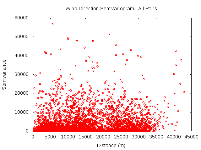
Variogram cloud showing wind direction
The first plot displays the semivariance of all pairs of schools. Unfortunately, it is difficult to discern any of the important properties (i.e., the nugget, range and sill) from this plot. Maybe the semivariogram would be more illuminating…
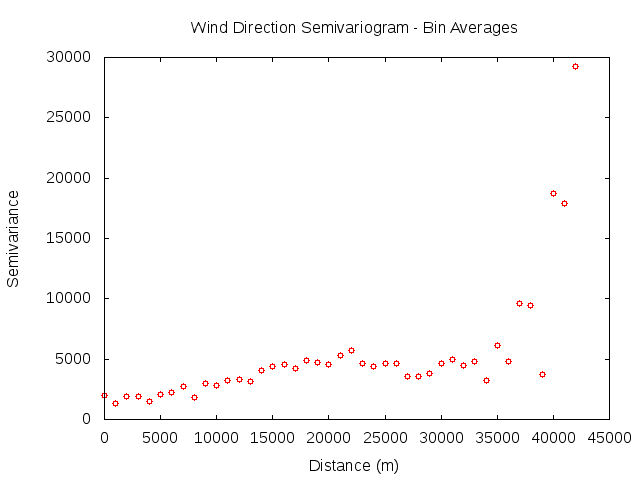
Semivariogram showing wind direction
More illuminating, but perhaps not in the way I had hoped. This plot indicates that the data follow a linear trend, known as drift. For ordinary Kriging, the assumption is that the mean value of the field is uniform, so that strategy is immediately eliminated. However, in universal Kriging, a trend surface is created to represent this drift and the analysis is performed on the residuals (O’Sullivan and Unwin, 2012).
The next post will examine universal Kriging and attempt to apply it to this problem.
Were you able to fit a curve to the variogram? It is linearish, but I think there is a range at 2300? Another super simple method would be to use Voronoi’s to interpolate. The key benefit would be that you would retain the exact values of the data when you use it as input to your resistance models. One other thing that I just thought of… climatologists have a lot of really specific guidelines for setting up weather stations, often based on height of towers. These are invalidated by the school network. But, for your work, you are interested in what happens about 3-4 ft above the road. The wind properties may be different. More just a note to think about. I love the idea of a network of citizens with little wind sensors on their bikes that record wind when the bike is stopped
Great job on the blog so far! Nicely put together.